Exploration numérique

Riemann Lab

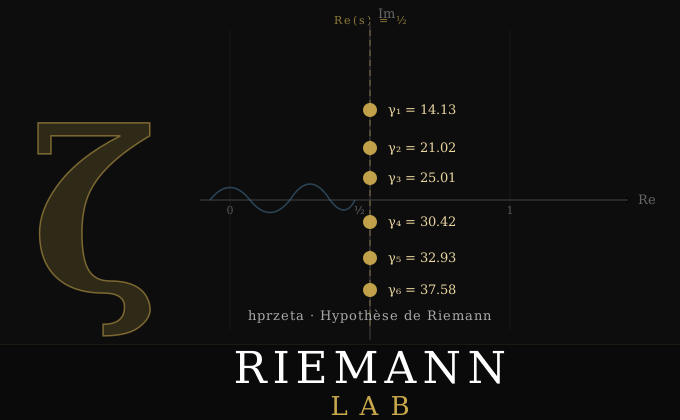
Laboratoire d'exploration de l'Hypothèse de Riemann — calcul des zéros non triviaux de $\zeta(s)$ sur la droite critique $\text{Re}(s) = \tfrac{1}{2}$.

Ubuntu 24.04 Python · mpmath 138 069 zéros validés · v16 · 0 manquant ✅ · Obj2 atteint 04/07/2026, amélioré 08/08/2026

$\zeta(s) = \displaystyle\sum_{n=1}^{\infty} \frac{1}{n^s}$ · $\text{Re}(s) = \tfrac{1}{2}$ · $Z(t) = e^{i\theta(t)}\,\zeta\!\left(\tfrac{1}{2}+it\right) \in \mathbb{R}$ · $\theta(t) = \text{Im}\!\left[\ln\Gamma\!\left(\tfrac{1}{4}+\tfrac{it}{2}\right)\right] - \tfrac{t}{2}\ln\pi$ · $\zeta(2) = \dfrac{\pi^2}{6} \approx 1.6449$ · $N(T) \approx \dfrac{T}{2\pi}\ln\!\dfrac{T}{2\pi e}$ · $\zeta(s) = \displaystyle\sum_{n=1}^{\infty} \frac{1}{n^s}$ · $\text{Re}(s) = \tfrac{1}{2}$ · $Z(t) = e^{i\theta(t)}\,\zeta\!\left(\tfrac{1}{2}+it\right) \in \mathbb{R}$ · $\theta(t) = \text{Im}\!\left[\ln\Gamma\!\left(\tfrac{1}{4}+\tfrac{it}{2}\right)\right] - \tfrac{t}{2}\ln\pi$ · $\zeta(2) = \dfrac{\pi^2}{6} \approx 1.6449$ · $N(T) \approx \dfrac{T}{2\pi}\ln\!\dfrac{T}{2\pi e}$ ·

Visualisation interactive — $\theta(t)$ de Riemann-Siegel

Animation de la fonction de phase $\theta(t)$ et de son rôle dans la détection des zéros de $\zeta\!\left(\tfrac{1}{2}+it\right)$ par changement de signe de $Z(t)$.

▶ Ouvrir l'animation GitHub → Wiki →

Animations interactives

∑ Série de Dirichlet Convergence $\zeta(s)=\sum 1/n^s$ selon $\text{Re}(s)$. Slider $\sigma$ + N termes. ↗ ∏ Produit eulérien Convergence $\prod(1-p^{-s})^{-1}$ vers $\zeta(s)$ premier par premier. ↗ ℂ Plan complexe Heatmap $|\zeta(\sigma+it)|$, pôle $s=1$, bande critique, zéros visibles. ↗ Γ Fonction Gamma Pôles aux entiers négatifs, formule de réflexion, lien avec $\xi(s)$. ↗ ⊞ Distribution des zéros Espacements normalisés, loi de Wigner (GUE) vs Poisson, $N(T)$ interactif. ↗ θ θ(t) — Cours complet Définition, Stirling, équation fonctionnelle, Backlund — 3 animations simultanées. ↗

138 069 zéros validés

10⁻¹⁵ précision max

99 999 t max atteint

Avancement du projet

Calcul des zéros non triviaux

v16 opérationnel — Illinois hybride 2-phases + cache RS 33 KB + Phase 2 adaptative (SEUIL_1NEWTON=20k) + Z_arb à précision fixe (acb_dirichlet_hardy_z, 64 bits, remplace l'escalade automatique arb_fpwrap ~1e-16 surdimensionnée vs le besoin réel 1e-12). 138 069 zéros calculés jusqu'à T=100 000 en 1.6 min · 1407 z/s (avec turbo) · 0 manquant. Turing-Backlund COMPLET ✅ · LMFDB 20/20 ✅ · ×2.75 vs v15 · ×787.5 vs v1.

Opérationnel — v16 ⭐ · Objectif 2 largement dépassé ✅

138 069
zéros ✓

Visualisations avancées

8 animations interactives en ligne — $\theta(t)$, $Z(t)$, plan $\mathbb{C}$, Gamma, Dirichlet, produit eulérien, distribution des zéros, mur de latence.

8 animations en ligne

En ligne

Intelligence artificielle locale

BrainVault structuré — inbox-ia opérationnel, 26 pavés ingérés (PDF → MD). Ollama + Mathstral : exploratoire. RAG non encore opérationnel.

Exploratoire

WIP

Preuves formelles Lean 4

Formalisation des résultats numériques en preuves mathématiques vérifiées par Lean 4.

Non démarré

○

Premiers zéros calculés

#	Partie imaginaire $t$	$\left\|\zeta\left(\tfrac{1}{2}+it\right)\right\|$	vs LMFDB
1	14.134725141734693	1.23e-14	✓ 0.00e+00
2	21.022039638771556	2.45e-14	✓ 0.00e+00
3	25.010857580145688	3.67e-14	✓ 0.00e+00
4	30.424876125859513	4.89e-14	✓ 0.00e+00
5	32.935061587739190	5.12e-14	✓ 0.00e+00
6	37.586178158825671	6.34e-14	✓ 7.11e-15
… 10 142 zéros supplémentaires jusqu'à t ≈ 10 000 zeros_T10000_10142.csv ↗

📚 Formation ζ & HR — du lycée au doctorat

Cours gradué en 14 chapitres — analyse complexe, fonction ζ, Hypothèse de Riemann. Chaque chapitre : démonstration, exemple numérique recalculé, piège/limite, lien avec le LAB.
« Lire » ouvre le chapitre sur le wiki · « PDF VAULT » télécharge le cours complet.

Chapitre 1 Série de Dirichlet & convergence